Fuel Cell Equilibrium¶

For the fuel cell shown in Figure 2.1.2, we want to determine its voltage at the open circuit condition (i.e., the current does not flow through the circuit due to a break in the circuit). The open circuit condition simplifies our calculation since any non-zero current would lead to a change in voltage due to resistance in the fuel cell (on the zeroth order, one can rationalize such change in voltage with Ohm’s law, $\Delta V=\Delta I\cdot R$). An open circuit can be achieved by removing the lightbulb in in Figure 2.1.2 to create a gap in the circuit. To use the generalized expression for chemical equilibrium as seen in Equation 2.4.6, we first need to figure out all species in a fuel cell that are relevant to chemical equilibrium.

Table 2.5.1 lists all species and chemical reactions in the fuel cell as shown in Figure 2.1.2. The subscripts denote whether the reaction is taking place at the cathode (C) or the anode (A). An extra note on the $1^{\text{st}}$ and $2^{\text{nd}}$ reactions, technically speaking, they are not chemical reactions, but rather transport processes. At open circuit, for a chemical reaction in the fuel cell to reach equilibrium, it needs to have a participating species that can traverse across the membrane/circuit to allow the forward and reverse reactions to equilibrate, namely $\text{O}^{2-}$ in this case. As a result, only the $1^{\text{st}}$, $3^{\text{rd}}$, and $4^{\text{th}}$ reactions can equilibrate. The remaining reactions cannot equilibrate because the species are physically separated. For the $2^{\text{nd}}$ reaction, electrons cannot flow through the broken circuit gap. The $5^{\text{th}}$ reaction represents the overall reaction of the fuel cell, where the gaseous species and water are blocked by the membrane. In summary, to calculate the open-circuit voltage of the fuel cell, we need to consider the following three reactions at equilibrium:

1. $2 \text{H}_2 + 2 \text{O}^{2-}_{\text{A}} \Leftrightarrow 2\text{H}_2\text{O} + 4 e^{-}_{\text{A}}$
2. $\text{O}_2 + 4 e^{-}_{\text{C}} \Leftrightarrow 2\text{O}^{2-}_{\text{C}}$
3. $\text{O}^{2-}_{\text{A}} \Leftrightarrow \text{O}^{2-}_{\text{C}}$

Applying the equilibrium condition from Equation 2.4.6, we obtain

1. $-2 \mu_{\text{H}_2} -2 \mu_{\text{O}^{2-}_{\text{A}}} + 2\mu_{\text{H}_2\text{O}} + 4\mu_{e^{-}_{\text{A}}} = 0$
2. $-\mu_{\text{O}_2} - 4 \mu_{e^{-}_{\text{C}}} + 2\mu_{\text{O}^{2-}_{\text{C}}}=0$
3. $-\mu_{\text{O}^{2-}_{\text{A}}} + \mu_{\text{O}^{2-}_{\text{C}}}=0$

The goal here is to to obtain the chemical potential difference between electrons in the cathode and the anode as a function of the chemical potentials of species in the overall $5^{\text{th}}$ reaction. The first step is to rearrange the equations as follows

1. $- 4\mu_{e^{-}_{\text{A}}} = -2 \mu_{\text{H}_2} -2 \mu_{\text{O}^{2-}_{\text{A}}} + 2\mu_{\text{H}_2\text{O}}$
2. $4 \mu_{e^{-}_{\text{C}}} = -\mu_{\text{O}_2} + 2\mu_{\text{O}^{2-}_{\text{C}}}$
3. $0=\mu_{\text{O}^{2-}_{\text{C}}} - \mu_{\text{O}^{2-}_{\text{A}}}$ or $\mu_{\text{O}^{2-}_{\text{C}}}=\mu_{\text{O}^{2-}_{\text{A}}}$

We then combine these three equations to have

We can see that the chemical potential of oxygen ions in the cathode cancels out that in the anode, which makes intuitive sense since they are the same chemical species, just placed in different part of the fuel cell. Normalizing the factor on the left hand side to be one, we obtain

From Equation 2.5.2, we can see that the electron chemical potential difference in the cathode and the anode is equal to a quarter of the chemical potential difference between the product ($\text{H}_2\text{O}$) and the reactants ($\text{H}_2$, $\text{O}_2$) in the overall fuel cell equation, multiplied by their respective stoichiometric coefficient. The factor of $1/4$ reflects that 4 electrons must be transferred from the anode to the cathode for every mole of oxygen gas consumed, assuming a closed circuit. To reiterate, at open circuit, the electron chemical potential difference between the cathode and the anode is precisely balanced by the chemical potential difference between the overall products and reactants in the fuel cell, weighted by their stoichiometric coefficients. Again, since charged ions are involved, we have omitted the electrostatic potential for simplicity.

Partial Molar Quantities¶

As discussed in previous sections, when the pressure and temperature of a system is held constant, the relevant thermodynamic potential is the Gibbs free energy. Starting from the derived equation of $G=H-TS$ and Equation 2.3.19, we have

Utilizing the notation introduced in Equation 2.5.4 on Equation 2.5.3, we get

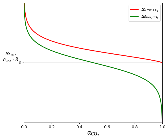
where $h_i$ relates to the change in the bond energy of the molecules/materials, and $s_i$ relates to the degree of randomness in the molecules. A more rigorous way to define partial molar enthalpy is as the infinitesimal change in a system’s enthalpy when an infinitesimal amount of species $i$ is added or removed, at constant $T$ and $P$. Similarly, the partial molar enthalpy is the infinitesimal change in a system’s entropy as the species $i$ is added to or removed from the system by an infinitesimal amount, at constant $T$ and $P$. Using the $\text{CO}_2$ separation as an example: the partial molar change in entropy of mixing is $\Delta s_{\text{mix, CO}_2}=\frac{\partial \Delta S_{\text{mix}}}{\partial n_{\text{CO}_2}}$, whereas the specific change of entropy of mixing is $\Delta \overline{S}_{\text{mix, CO}_2}=\frac{\Delta S_{\text{mix}}}{n_{\text{CO}_2}}$, denoted by the green and red line in the following plot, respectively. (Note: here we are showing partial molar change in entropy of mixing, but we can also define a partial molar entropy for processes without mixing)

Source:Partial Molar Entropy

A more general comparison between a specific quantity and a partial molar quantity can be found in Figure 2.5.2. The specific quantity can be thought of as an aggregate slope of $Y/X$, whereas the partial molar quantity is the tangent slope of $\dd Y/\dd X$.