APMC2025 | 4D-STEM workshop

Georgios Varnavides

Workshop

Contents

Our goal is to perform automated crystal orientation mapping (ACOM), as described in:
Automated Crystal Orientation Mapping in py4DSTEM using Sparse Correlation Matching

Data¶

polycrystal_2D_WS2.h5 (1.0 GB)

WS2.cif (2 kB)

This dataset is a simulation of a polycrystalline WS2 thin film, where each grain has an [0001] zone axis orientation, and a random in-plane rotation. Each grain has been randomly strained by -2%, -1%, 0%, 1%, or 2%, for e_xx, e_yy, and e_xy. This makes checking the output strain maps easier, as each grain has an exact multiple of 1% strain for each value in the strain tensor. The dataset for this tutorial has also been downsampled in both real and diffraction space to make a small example.

pymatgen¶

This notebook requires that pymatgen is installed.

Colin Ophus (clophus@lbl.gov)
Alex Rakowski (arakowski@lbl.gov)
Stephanie Ribet (sribet@lbl.gov)
Ben Savitzky (bhsavitzky@lbl.gov)
Steve Zeltmann (steven.zeltmann@berkeley.edu)

Last updated: 2025 Feb 01

%pip install py4DSTEM pymatgen > /dev/null 2>&1

import py4DSTEM
import numpy as np

print(py4DSTEM.__version__)
%matplotlib inline

cupyx.jit.rawkernel is experimental. The interface can change in the future.

0.14.18

Download and import data¶

# Get the 4DSTEM data and cif file
py4DSTEM.io.gdrive_download(
    id_ = 'https://drive.google.com/uc?id=13zBl6aFExtsz_sew-L0-_ALYJfcgHKjo',
    destination = '/content/',
    filename = 'WS2.cif',
    overwrite=True
)
py4DSTEM.io.gdrive_download(
    id_ = 'https://drive.google.com/uc?id=1AWB3-UTPiTR9dgrEkNFD7EJYsKnbEy0y',
    destination = '/content/',
    filename = 'polycrystal_2D_WS2.h5',
    overwrite=True
)

Downloading...
From: https://drive.google.com/uc?id=13zBl6aFExtsz_sew-L0-_ALYJfcgHKjo
To: /content/WS2.cif
100%|██████████| 2.37k/2.37k [00:00<00:00, 4.98MB/s]
Downloading...
From (original): https://drive.google.com/uc?id=1AWB3-UTPiTR9dgrEkNFD7EJYsKnbEy0y
From (redirected): https://drive.google.com/uc?id=1AWB3-UTPiTR9dgrEkNFD7EJYsKnbEy0y&confirm=t&uuid=174181a2-085d-4827-a4f4-d3cc6fe3e866
To: /content/polycrystal_2D_WS2.h5
100%|██████████| 1.07G/1.07G [00:16<00:00, 64.2MB/s]

# Local pathways to  data and crystal structure
filepath_data = '/content/polycrystal_2D_WS2.h5'
filepath_cif = '/content/WS2.cif'

py4DSTEM.print_h5_tree(filepath_data)

/
|---4DSTEM
    |---datacube
        |---calibration

# Load the datacube using py4DSTEM
dataset = py4DSTEM.read(
    filepath_data,
    root='4DSTEM/datacube',
)

Virtual imaging¶

dataset.get_dp_max()
dataset.get_dp_mean()

VirtualDiffraction( A 2-dimensional array of shape (128, 128) called 'dp_mean',
                    with dimensions:

                        dim0 = [0,1,2,...] pixels
                        dim1 = [0,1,2,...] pixels
)

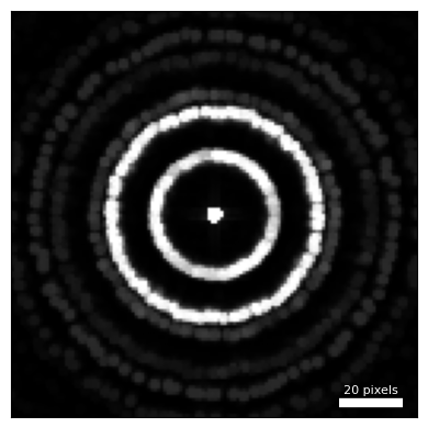
py4DSTEM.visualize.show(
    dataset.tree('dp_max'),
    figsize = (4,4),
    ticks = False,
)

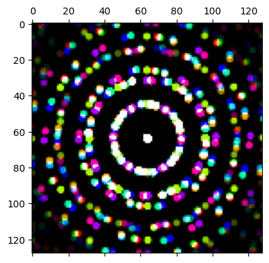
py4DSTEM.show(
    [
        dataset.data[20,20],
        dataset.data[90,20],
        dataset.data[120,20],
        dataset.data[20,70],
        dataset.data[50,70],
        dataset.data[90,70],
        dataset.data[20,110],
        dataset.data[70,110],
        dataset.data[110,110],
    ],
    combine_images=True,
    figsize = (4,4),
)

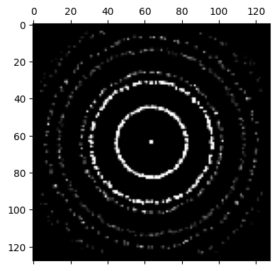
We can see the polycrystalline grain structure of the WS2 in the maximum diffraction pattern. Many diffraction rings are present, with Bragg peaks at many different rotations along these rings.

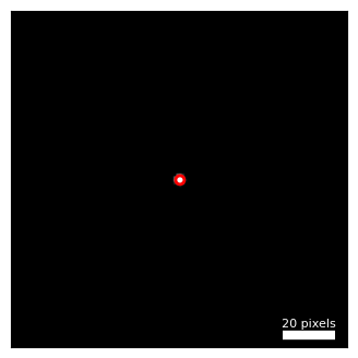
# Estimate the radius of the BF disk, and the center coordinates
probe_semiangle, probe_qx0, probe_qy0 = dataset.get_probe_size(
    dataset.tree('dp_mean').data,
    thresh_lower = 0.5,
)
center = (probe_qx0, probe_qy0)

# plot the mean diffraction pattern, with the estimated probe radius overlaid as a circle
fig, ax = py4DSTEM.show(
    dataset.tree('dp_mean'),
    figsize=(4,4),
    circle = {
        'center': center,
        'R': probe_semiangle,
    },
    ticks = False,
    returnfig = True,
    vmax = 1,
);
# ax.set_xlim([57, 70]);
# ax.set_ylim([70, 57]);

# Print the estimate probe radius
print('Estimated probe radius =', '%.2f' % probe_semiangle, 'pixels')

Estimated probe radius = 1.64 pixels

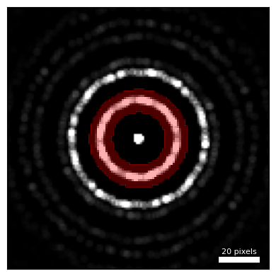
# Create a virtual annular dark field (ADF) image around the first diffraction ring

radii = (13,24)

# Plot the ADF detector
dataset.position_detector(
    mode = 'annular',
    geometry = (
        center,
        radii
    ),
    figsize = (4,4),
    ticks = False,
)

# Calculate the ADF image
dataset.get_virtual_image(
    mode = 'annulus',
    geometry = (center,radii),
    name = 'dark_field',
)

# Plot the ADF image
py4DSTEM.show(
    dataset.tree('dark_field'),
    figsize = (4,4),
)

100%|██████████| 16384/16384 [00:00<00:00, 18586.28it/s]

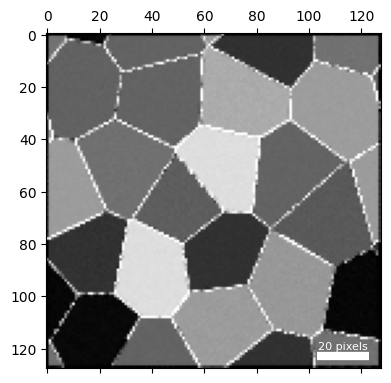
Two kinds of contrast changes are visible in the virtual dark field image:

The grain boundaries show up as bright lines bordering the polycrystalline grains.
Some grains appear brighter or darker - this is because the applied strain fields increase or decrease the atomic density of the grains, leading to more or less diffraction into the annular dark field region.

Probe template¶

# Because the diffracted signal is so weak, we will just average a subset of the probe positions.
rx_min, rx_max = 10, 50
ry_min, ry_max = 10, 50

probe = dataset.get_vacuum_probe(
    ROI=(rx_min, rx_max, ry_min, ry_max),
    threshold = 1e-5,
    #mask,
    #align=True,
)

100%|██████████| 1599/1599 [00:05<00:00, 316.37it/s]

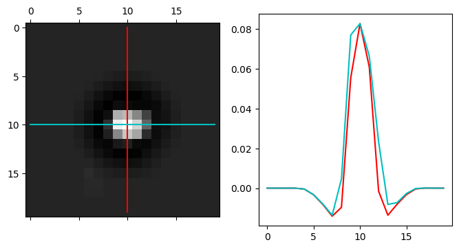
# Subtract a normalization function to give the probe a mean value of zero
probe.get_kernel(
    mode = 'sigmoid',
    radii = (probe_semiangle * 0.0, probe_semiangle * 4.0),
    bilinear=True,
)

# Plot the probe kernel
py4DSTEM.visualize.show_kernel(
    probe.kernel,
    R=10, L=10, W=1,
    figsize = (8,4),
)

Bragg disk detection¶

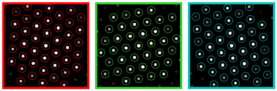
# Test parameters on a few probe positions
# Visualize the diffraction patterns and the located disk positions

rxs = 32,96,96
rys = 32,32,96
colors=['r','limegreen','c']


# parameters
detect_params = {
    'corrPower': 1.0,
    'sigma': 0,
    'edgeBoundary': 4,
    'minRelativeIntensity': 0,
    'minAbsoluteIntensity': 4e-7,
    'minPeakSpacing': 12,
    'subpixel' : 'poly',
#     'subpixel' : 'multicorr',
    'upsample_factor': 8,
    'maxNumPeaks': 1000,
#     'CUDA': True,
}

disks_selected = dataset.find_Bragg_disks(
    data = (rxs, rys),
    template = probe.kernel,
    **detect_params,
)

py4DSTEM.visualize.show_image_grid(
    get_ar = lambda i:dataset.data[rxs[i],rys[i],:,:],
    H=1,
    W=3,
    axsize=(3,3),
    get_bordercolor = lambda i:colors[i],
    get_x = lambda i: disks_selected[i].data['qx'],
    get_y = lambda i: disks_selected[i].data['qy'],
    get_pointcolors = lambda i: colors[i],
    open_circles = True,
    scale = 300,
)

# Find Bragg peaks for all probe positions
bragg_peaks = dataset.find_Bragg_disks(
    template = probe.kernel,
    **detect_params,
)

Finding Bragg Disks: 100%|██████████| 16.4k/16.4k [00:58<00:00, 278DP/s]

Centering and calibration¶

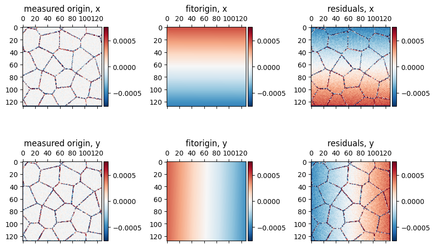
# Compute the origin position for all probe positions by finding and then fitting the center beam

# measure origins
qxy_origins = bragg_peaks.measure_origin(
    # mode = 'no_beamstop',
)

# fit a plane to the origins
qx0_fit,qy0_fit,qx0_residuals,qy0_residuals = bragg_peaks.fit_origin(
    # plot_range=0.1,
    figsize = (4,4)
)

# Calculate BVM from centered data
bragg_vector_map_centered = bragg_peaks.get_bvm()

py4DSTEM.show(
    bragg_vector_map_centered,
    figsize = (4,4),
)

Pixel size calibration¶

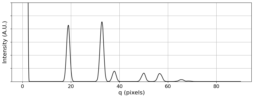
# Calculate and plot the radial integral.
# Note that for a 2D material, the center beam is orders of magnitude higher than the diffracted beam.
# Thus we need to specify a maximum y value for the plot.
# We also scale the plotted intensity by q to better show the higher angle peaks.
ymax = 30

q, intensity_radial = py4DSTEM.process.utils.radial_integral(
    bragg_vector_map_centered,
)

py4DSTEM.visualize.show_qprofile(
    q = q,
    intensity = intensity_radial * q,
    ymax = ymax,
)

# Load the WS2 crystal file
crystal = py4DSTEM.process.diffraction.Crystal.from_CIF(filepath_cif)

get_structures is deprecated; use parse_structures in pymatgen.io.cif instead.
The only difference is that primitive defaults to False in the new parse_structures method.So parse_structures(primitive=True) is equivalent to the old behavior of get_structures().
Issues encountered while parsing CIF: 4 fractional coordinates rounded to ideal values to avoid issues with finite precision.

# Calculate structure factors
k_max = 1.4

crystal.calculate_structure_factors(
    k_max,
)

crystal.plot_structure(
    zone_axis_lattice=(1,1,0.1),
    figsize=(6,3),
    camera_dist = 6,
)

# Test different pixel sizes, and overlay the structure factors onto the experimental data.
# Note that we will use our knowledge that the WS2 has an [0001] zone axis.

inv_Ang_per_pixel = 0.0192

q_SF = np.linspace(0,k_max,250)
I_SF = np.zeros_like(q_SF)
for a0 in range(crystal.g_vec_leng.shape[0]):
    if np.abs(crystal.g_vec_all[2,a0]) < 0.01:
        idx = np.argmin(np.abs(q_SF-crystal.g_vec_leng[a0]))
        I_SF[idx] += crystal.struct_factors_int[a0]
I_SF /= np.max(I_SF)

fig,ax = py4DSTEM.visualize.show_qprofile(
    q=q*inv_Ang_per_pixel,
    intensity=intensity_radial*q,
    xlabel='q (1/Ang)',
    returnfig=True,
    ymax=ymax,
)

ax.plot(q_SF,I_SF*ymax,c='r')
ax.set_xlim([0, k_max])

(0.0, 1.4)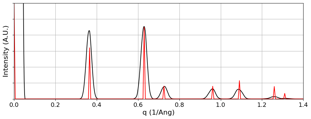

# Apply pixel size calibration
bragg_peaks.calibration.set_Q_pixel_size(inv_Ang_per_pixel)
bragg_peaks.calibration.set_Q_pixel_units('A^-1')

bragg_peaks.calstate

{'center': True, 'ellipse': False, 'pixel': True, 'rotate': False}

# Save calibrated Bragg peaks
filepath_braggdisks_cal = '/content/braggdisks_cal.h5'
py4DSTEM.save(
    filepath_braggdisks_cal,
    bragg_peaks,
    mode='o',
)

100%|██████████| 16384/16384 [00:02<00:00, 6300.75it/s]

Automated crystal orientation mapping (ACOM)¶

# Reload Bragg peaks if needed
# filepath_braggdisks_cal = '/content/braggdisks_cal.h5'
# py4DSTEM.print_h5_tree(filepath_braggdisks_cal)

# Reload bragg peaks cif file, recompute structure factors
# bragg_peaks = py4DSTEM.read(
#     filepath_braggdisks_cal,
# )
# bragg_peaks

k_max = 1.4
crystal = py4DSTEM.process.diffraction.Crystal.from_CIF(filepath_cif)
crystal.calculate_structure_factors(
    k_max,
)

get_structures is deprecated; use parse_structures in pymatgen.io.cif instead.
The only difference is that primitive defaults to False in the new parse_structures method.So parse_structures(primitive=True) is equivalent to the old behavior of get_structures().
Issues encountered while parsing CIF: 4 fractional coordinates rounded to ideal values to avoid issues with finite precision.

# Create an orientation plan for [0001] WS2
crystal.orientation_plan(
    angle_step_zone_axis = 1.0,
    angle_step_in_plane = 4.0,
    zone_axis_range = 'fiber',
    fiber_axis = [0,0,1],
    fiber_angles = [0,0],

    corr_kernel_size = 0.16,
#     CUDA=True,
)

Orientation plan: 100%|██████████| 1/1 [00:00<00:00, 535.60 zone axes/s]

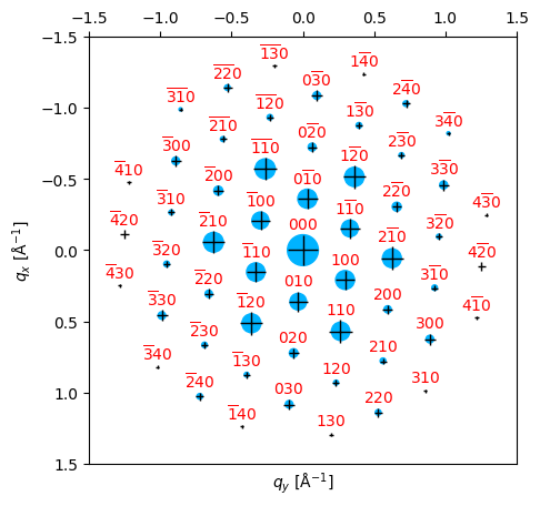
# Test matching on some probe positions
# xind, yind = 64,64
xind, yind= 32,96
xind, yind= 20,45

orientation  = crystal.match_single_pattern(
    bragg_peaks.cal[xind,yind],
#     plot_corr = True,
#     plot_polar = False,
    verbose = True,
)

sigma_compare = 0.02
range_plot = np.array([k_max+0.1,k_max+0.1])

bragg_peaks_fit = crystal.generate_diffraction_pattern(
    orientation,
    ind_orientation=0,
    sigma_excitation_error=sigma_compare)


# plot comparisons
py4DSTEM.process.diffraction.plot_diffraction_pattern(
    bragg_peaks_fit,
    bragg_peaks_compare=bragg_peaks.cal[xind,yind],
    scale_markers=1e4,
    scale_markers_compare=1e7,
    plot_range_kx_ky=range_plot,
    min_marker_size=1,
    max_marker_size=400,
    figsize = (5,5),
)

Best fit lattice directions: z axis = ([ 0.  0. -0. -1.]), x axis = ([ 0.485 -0.048 -0.437  0.   ]), with corr value = 0.273

# Fit orientation to all probe positions
orientation_map = crystal.match_orientations(
    bragg_peaks,
    inversion_symmetry = False,
)

Warning: bragg peaks not elliptically calibrated
bragg peaks not rotationally calibrated
Matching Orientations: 100%|██████████| 16384/16384 [01:58<00:00, 138.26 PointList/s]

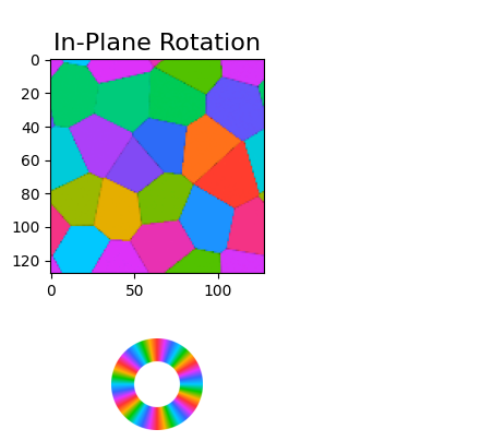
# Plot the orientations
images_orientation = crystal.plot_fiber_orientation_maps(
    orientation_map,
    symmetry_order = 6,
    corr_range = [0.0, 1.0],
    figsize = (4,4),
)

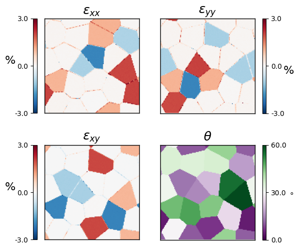
Strain maps¶

For each diffraction pattern, we have both the measured diffraction pattern Bragg peaks, and the Bragg peaks calculated from the best-fit orientation. We can therefore directly calculate a strain map, just by measuring the best-fit transformation tensor between these two sets of peaks.

strain_map = crystal.calculate_strain(
    bragg_peaks,
    orientation_map,
    rotation_range=np.pi/3, # 60 degrees
#     corr_kernel_size=0.02,
)

bragg peaks not elliptically calibrated
bragg peaks not rotationally calibrated
Calculating strains: 100%|██████████| 16384/16384 [00:32<00:00, 510.04 PointList/s]

# plot the 4 components of the strain tensor
fig,ax = py4DSTEM.visualize.show_strain(
    strain_map,
    vrange_exx=[-3.0, 3.0],
    vrange_theta=[0.0, 60.0],
    ticknumber=3,
    # axes_plots=(),
    # bkgrd=False,
    figsize=(6,6),
#     cmap='hsv',
    returnfig=True,
    # cmap_theta = 'hsv',
)

Acknowledgments¶

This tutorial was created by the py4DSTEM instructor team:

References¶

Ophus, C., Zeltmann, S. E., Bruefach, A., Rakowski, A., Savitzky, B. H., Minor, A. M., & Scott, M. C. (2022). Automated Crystal Orientation Mapping in py4DSTEM using Sparse Correlation Matching. Microscopy and Microanalysis, 28(2), 390–403. 10.1017/s1431927622000101

Try it Yourself!

Dynamical Diffraction Tutorial 01

Try it Yourself!

Orientation Mapping Tutorial