Direct Ptychography Tutorial 03

This is the third and last tutorial notebook in the direct ptychography series.
In this tutorial notebook we will cover:
- Optimum bright-field STEM reconstructions
- Wigner distribution deconvolution reconstructions
- Segmented-detector reconstructions
Downloads
This tutorial uses the following datasets:
- Georgios Varnavides (gvarnavides@berkeley
.edu) - Stephanie Ribet (sribet@lbl.gov)
- Colin Ophus (cophus@stanford.edu)
Last updated: 2024 Feb 01
Introduction
So far, we have only used the (phase-compensated) single-side band (SSB) method. There are two closely-related techniques which have been proposed to perform better for low-dose datasets. Those are:
- Optimum bright-field (OBF) STEM: [Ooe, K., et al. (2021), Ultramic, 220, 113133]
- Wigner distribution deconvolution (WDD): [Yang, H., et al. (2017), Ultramic, 180, 173-179]
%pip install py4DSTEM > /dev/null 2>&1import numpy as np
import py4DSTEM
import matplotlib.pyplot as plt
print(py4DSTEM.__version__)
%matplotlib inlinecupyx.jit.rawkernel is experimental. The interface can change in the future.
0.14.18
We’ll use the same, in-focus, dataset as the one we used in direct_ptychography_01.ipynb.
# Get the 4DSTEM data
py4DSTEM.io.gdrive_download(
    id_ = 'https://drive.google.com/uc?id=1Ml1Ga4-U0ZcTJxq0LVyTJDIVfnBuyd81',
    destination = '/content/',
    filename = 'dpc_STO_simulation.h5',
    overwrite=True
)
Downloading...
From: https://drive.google.com/uc?id=1Ml1Ga4-U0ZcTJxq0LVyTJDIVfnBuyd81
To: /content/dpc_STO_simulation.h5
100%|██████████| 75.5M/75.5M [00:00<00:00, 139MB/s]
file_path = '/content/'
file_data = file_path + 'dpc_STO_simulation.h5'

dataset = py4DSTEM.read(file_data)
dataset.crop_Q((24,-24,24,-24))
DataCube( A 4-dimensional array of shape (32, 32, 48, 48) called 'datacube',
with dimensions:
Rx = [0.0,0.12328531250000001,0.24657062500000002,...] A
Ry = [0.0,0.12328531250000001,0.24657062500000002,...] A
Qx = [0.0,1.0595062826244177,2.1190125652488354,...] mrad
Qy = [0.0,1.0595062826244177,2.1190125652488354,...] mrad
)SSB Algorithm Variants
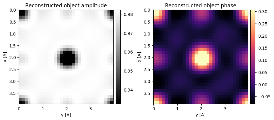
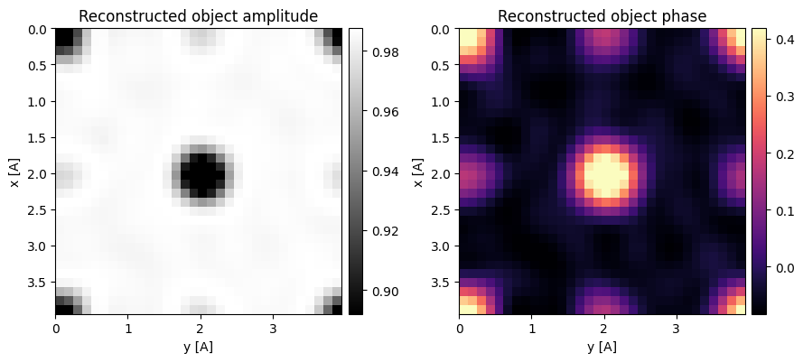
First, let’s reproduce the phase-compensated SSB reconstruction from direct_ptychography_01.ipynb:
energy = 200e3
semiangle_cutoff = 20

ssb = py4DSTEM.process.phase.SSB(
    energy=energy,
    datacube=dataset,
    semiangle_cutoff=semiangle_cutoff,
    verbose=True,
).preprocess(
    plot_center_of_mass=False,
    plot_rotation=False,
    plot_overlap_trotters=False,
    force_com_rotation=-15,
    crop_around_bf_disk=False,
).reconstruct(
).visualize(
)
Calculating center of mass: 100%|██████████| 1024/1024 [00:00<00:00, 8019.79probe position/s]
Best fit rotation forced to -15 degrees.
Normalizing amplitudes: 100%|██████████| 1024/1024 [00:01<00:00, 617.03probe position/s]
100%|██████████| 1024/1024 [00:02<00:00, 342.46it/s]
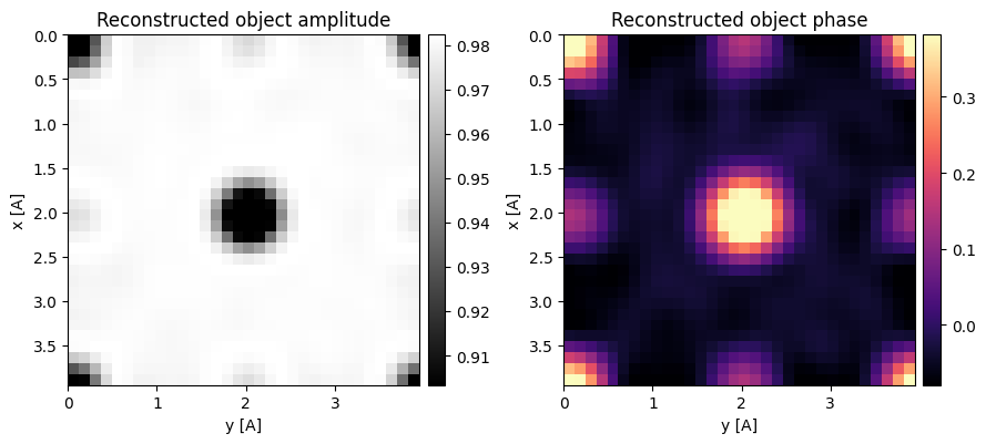
Optimum bright-field (OBF) STEM also compensates for the phase in the double minus triple overlap trotters, albeit using a different normalization.
In py4DSTEM, this can be invoked using the OBF class.
obf = py4DSTEM.process.phase.OBF(
    energy=energy,
    datacube=dataset,
    semiangle_cutoff=semiangle_cutoff,
    verbose=True,
).preprocess(
    plot_center_of_mass=False,
    plot_rotation=False,
    plot_overlap_trotters=False,
    force_com_rotation=-15,
    crop_around_bf_disk=False,
).reconstruct(
).visualize(
)
Calculating center of mass: 100%|██████████| 1024/1024 [00:00<00:00, 43286.88probe position/s]
Best fit rotation forced to -15 degrees.
Normalizing amplitudes: 100%|██████████| 1024/1024 [00:00<00:00, 2736.99probe position/s]
100%|██████████| 1024/1024 [00:01<00:00, 922.49it/s]
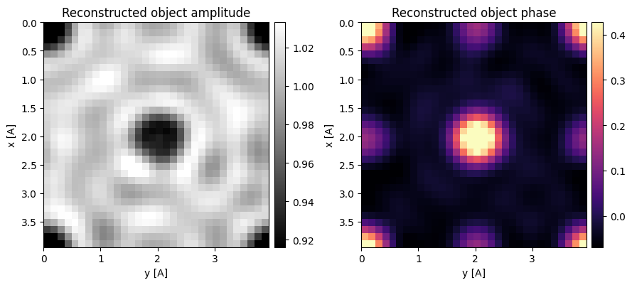
Wigner distribution deconvolution (WDD) is a more involved technique which attempts to fully deconvolve the effects of the probe from the object.
The method uses a Wiener-filter to avoid dividing by zero and boosting noise.
It can be invoked in py4DSTEM using the WDD class and requires the user specify the (relative) Wiener filtering parameter (with reasonable values between 0.01 - 0.1).
wdd = py4DSTEM.process.phase.WDD(
    energy=energy,
    datacube=dataset,
    semiangle_cutoff=semiangle_cutoff,
    verbose=True,
).preprocess(
    plot_center_of_mass=False,
    plot_rotation=False,
    plot_overlap_trotters=False,
    force_com_rotation=-15,
    crop_around_bf_disk=False,
).reconstruct(
    relative_wiener_epsilon=0.01,
).visualize(
)
Calculating center of mass: 100%|██████████| 1024/1024 [00:00<00:00, 45614.47probe position/s]
Best fit rotation forced to -15 degrees.
Normalizing amplitudes: 100%|██████████| 1024/1024 [00:00<00:00, 2819.14probe position/s]
100%|██████████| 1024/1024 [00:01<00:00, 1171.38it/s]
The reconstructions all look quite similar, with OBF and WDD showing (slightly) higher information limits
fig, axs = plt.subplots(2,3,figsize=(12,8))

for ax, arr, title in zip(
    axs[0],
    (np.angle(ssb.object),np.angle(obf.object),np.angle(wdd.object)),
    ('reconstructed phase (SSB)','reconstructed phase (OBF)','reconstructed phase (WDD)')
):
    py4DSTEM.show(
        np.tile(arr,(2,2)),
        figax=(fig,ax),
        cmap='turbo',
        ticks=False,
        title=title,
    )

for ax, arr in zip(
    axs[1],
    (np.angle(ssb.object),np.angle(obf.object),np.angle(wdd.object))
):
    py4DSTEM.show(
        np.tile(arr,(2,2)),
        figax=(fig,ax),
        cmap='turbo',
        show_fft=True,
        apply_hanning_window=False,
        ticks=False,
    )

fig.tight_layout()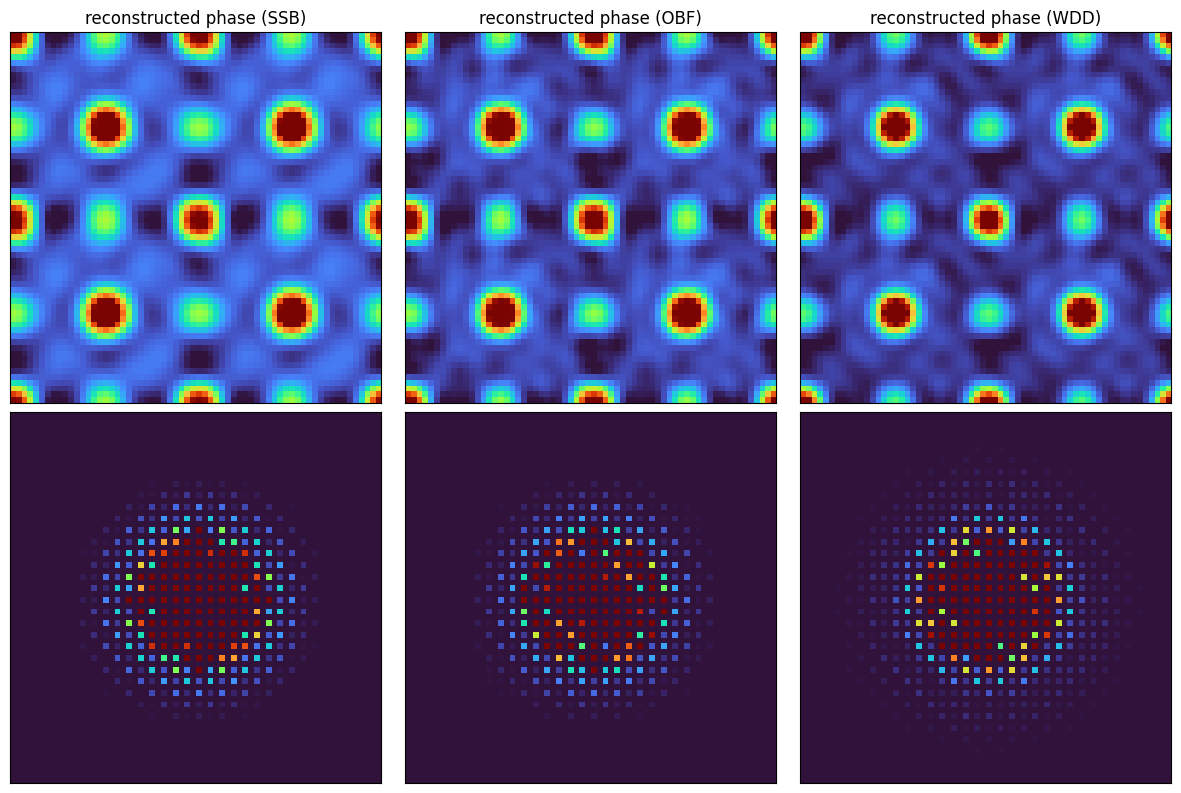
Segmented Detector Datasets
SSB and OBF are additionally very useful in post-processing segmented-detector datasets.
To see this, we’ll post-process our 4D-data using an annular detector with 6 segments.
def annular_segmented_detectors(
    energy,
    gpts,
    sampling,
    n_angular_bins,
    rotation_offset = 0,
    inner_radius = 0,
    outer_radius = np.inf,
):
    """ """
    nx,ny = gpts
    sx,sy = sampling
    wavelength = py4DSTEM.process.utils.electron_wavelength_angstrom(energy)

    alpha_x = np.fft.fftfreq(nx,sx)*wavelength
    alpha_y = np.fft.fftfreq(ny,sy)*wavelength

    alpha = np.sqrt(alpha_x[:,None]**2 + alpha_y[None,:]**2)
    radial_mask = ((inner_radius*1e-3 <= alpha) & (alpha < outer_radius*1e-3))

    theta = (np.arctan2(alpha_y[None,:], alpha_x[:,None]) + rotation_offset) % (2 * np.pi)
    angular_bins = np.floor(n_angular_bins * (theta / (2 * np.pi))) + 1
    angular_bins *= radial_mask.astype("int")

    angular_bins = [np.fft.fftshift((angular_bins == i).astype("int")) for i in range(1,n_angular_bins+1)]
    return angular_bins

def create_segmented_4d_dataset_using_virtual_detectors(dc,masks):
    """ """

    masks_np = np.array(masks).astype(np.bool_)

    preprocessed_data = np.zeros(dc.shape,dtype=np.float32)
    for mask in masks_np:
        val = np.sum(dc.data*mask,axis=(-1,-2)) / np.sum(mask)
        preprocessed_data[...,mask] = val[:,:,None]

    preprocessed_dataset = py4DSTEM.DataCube(preprocessed_data,calibration=dc.calibration.copy())
    return preprocessed_dataset

segmented_detector_masks = annular_segmented_detectors(
    energy=energy,
    gpts=dataset.Qshape,
    sampling=ssb.sampling,
    n_angular_bins = 4,
    inner_radius = semiangle_cutoff/2,
    outer_radius=semiangle_cutoff,
)

segmented_dataset = create_segmented_4d_dataset_using_virtual_detectors(dataset,segmented_detector_masks)
We plot the mean diffraction pattern alongside the segmented detector masks to emphasize the vast reduction in information encoded in this dataset:
fig, axs = plt.subplots(1,3,figsize=(12,4))

py4DSTEM.show(
    dataset.data.mean((0,1)),
    ticks=False,
    figax=(fig,axs[0]),
    title="mean diffraction pattern",
)

py4DSTEM.show(
    segmented_detector_masks,
    combine_images=True,
    ticks=False,
    figax=(fig,axs[1]),
    title="segmented detector masks",
)

py4DSTEM.show(
    segmented_dataset.data.mean((0,1)),
    combine_images=True,
    ticks=False,
    figax=(fig,axs[2]),
    title="mean segmented pattern",
    vmin=0,vmax=1,
)

fig.tight_layout()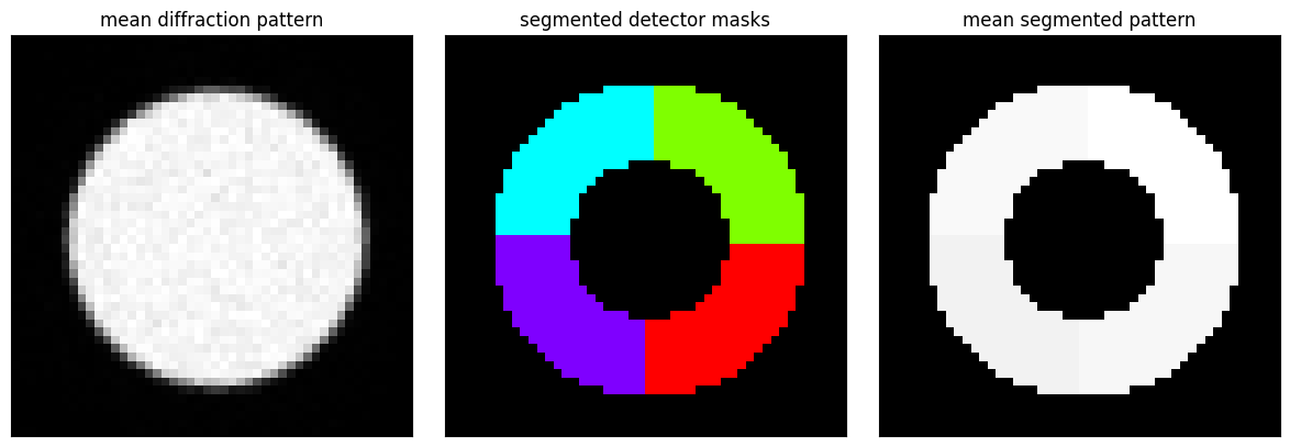
We can then use this pre-processed DataCube in the SSB and OBF classes, by passing a virtual_detector_masks argument in reconstruct.
Note this accepts “corner-centered” masks.
corner_centered_segmented_detector_masks = [np.fft.fftshift(mask.astype(np.bool_)) for mask in segmented_detector_masks]

segmented_ssb = py4DSTEM.process.phase.SSB(
    energy=energy,
    datacube=segmented_dataset,
    semiangle_cutoff=semiangle_cutoff,
    verbose=True,
).preprocess(
    plot_center_of_mass=False,
    plot_rotation=False,
    plot_overlap_trotters=False,
    force_com_rotation=-15,
    crop_around_bf_disk=False,
).reconstruct(
    virtual_detector_masks=corner_centered_segmented_detector_masks,
).visualize(
)
Calculating center of mass: 100%|██████████| 1024/1024 [00:00<00:00, 46086.31probe position/s]
Best fit rotation forced to -15 degrees.
Normalizing amplitudes: 100%|██████████| 1024/1024 [00:00<00:00, 2797.24probe position/s]
100%|██████████| 1024/1024 [00:01<00:00, 775.09it/s]

segmented_obf = py4DSTEM.process.phase.OBF(
    energy=energy,
    datacube=segmented_dataset,
    semiangle_cutoff=semiangle_cutoff,
    verbose=True,
).preprocess(
    plot_center_of_mass=False,
    plot_rotation=False,
    plot_overlap_trotters=False,
    force_com_rotation=-15,
    crop_around_bf_disk=False,
).reconstruct(
    virtual_detector_masks=corner_centered_segmented_detector_masks,
).visualize(
)
Calculating center of mass: 100%|██████████| 1024/1024 [00:00<00:00, 20018.12probe position/s]
Best fit rotation forced to -15 degrees.
Normalizing amplitudes: 100%|██████████| 1024/1024 [00:00<00:00, 1758.27probe position/s]
100%|██████████| 1024/1024 [00:02<00:00, 440.38it/s]
Indeed, the methods still work remarkably well!
fig, axs = plt.subplots(2,2,figsize=(8,8))

for ax, arr, title in zip(
    axs[0],
    (np.angle(segmented_ssb.object),np.angle(segmented_obf.object)),
    ('reconstructed phase (segmented SSB)','reconstructed phase (segmented OBF)')
):
    py4DSTEM.show(
        np.tile(arr,(2,2)),
        figax=(fig,ax),
        cmap='turbo',
        ticks=False,
        title=title,
    )

for ax, arr in zip(
    axs[1],
    (np.angle(segmented_ssb.object),np.angle(segmented_obf.object))
):
    py4DSTEM.show(
        np.tile(arr,(2,2)),
        figax=(fig,ax),
        cmap='turbo',
        show_fft=True,
        apply_hanning_window=False,
        ticks=False,
    )

fig.tight_layout()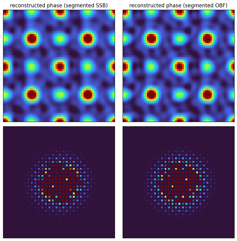
Acknowledgments
This tutorial was created by the py4DSTEM phase_contrast team:
- Ooe, K., Seki, T., Ikuhara, Y., & Shibata, N. (2021). Ultra-high contrast STEM imaging for segmented/pixelated detectors by maximizing the signal-to-noise ratio. Ultramicroscopy, 220, 113133. 10.1016/j.ultramic.2020.113133
- Yang, H., MacLaren, I., Jones, L., Martinez, G. T., Simson, M., Huth, M., Ryll, H., Soltau, H., Sagawa, R., Kondo, Y., Ophus, C., Ercius, P., Jin, L., Kovács, A., & Nellist, P. D. (2017). Electron ptychographic phase imaging of light elements in crystalline materials using Wigner distribution deconvolution. Ultramicroscopy, 180, 173–179. 10.1016/j.ultramic.2017.02.006

