Direct Ptychography Tutorial 02

This is the second tutorial notebook in the direct ptychography series.
In this tutorial notebook we will cover:
- Single side band (SSB) reconstructions with known aberrations
- Recursive aberration-fitting using the complex probe overlap function
Downloads
This tutorial uses the following datasets:
- Georgios Varnavides (gvarnavides@berkeley
.edu) - Stephanie Ribet (sribet@lbl.gov)
- Colin Ophus (cophus@stanford.edu)
Last updated: 2025 Feb 01
Introduction
The previous tutorial used an in-focus simulated dataset, to introduce the SSB and WDD algorithms.
In practice, as hard as we try and correct aberrations on the microscope -- our probe will have some residual aberrations.
%pip install py4DSTEM > /dev/null 2>&1import numpy as np
import py4DSTEM
import matplotlib.pyplot as plt
print(py4DSTEM.__version__)
%matplotlib inlinecupyx.jit.rawkernel is experimental. The interface can change in the future.
0.14.18
We load the dataset, which is very similar to the previous tutorial, but simulated using an aberrated probe.
# Get the 4DSTEM data
py4DSTEM.io.gdrive_download(
    id_ = 'https://drive.google.com/uc?id=1naukh3S54nvR-lkAH756ILEvs2JVXEyS',
    destination = '/content/',
    filename = 'dpc_STO_simulation_aberrated.h5',
    overwrite=True
)
Downloading...
From: https://drive.google.com/uc?id=1naukh3S54nvR-lkAH756ILEvs2JVXEyS
To: /content/dpc_STO_simulation_aberrated.h5
100%|██████████| 75.5M/75.5M [00:00<00:00, 91.0MB/s]
file_path = '/content/'
file_data = file_path + 'dpc_STO_simulation_aberrated.h5'

dataset = py4DSTEM.read(file_data)
dataset
DataCube( A 4-dimensional array of shape (32, 32, 96, 96) called 'datacube',
with dimensions:
Rx = [0.0,0.12328531250000001,0.24657062500000002,...] A
Ry = [0.0,0.12328531250000001,0.24657062500000002,...] A
Qx = [0.0,1.0595062826244177,2.1190125652488354,...] mrad
Qy = [0.0,1.0595062826244177,2.1190125652488354,...] mrad
)Effect of aberrations
First, let’s try and reconstruct like before -- to see the effect of aberrations on the reconstruction:
energy = 200e3
semiangle_cutoff = 20

ssb = py4DSTEM.process.phase.SSB(
    energy=energy,
    datacube=dataset,
    semiangle_cutoff=semiangle_cutoff,
    verbose=True,
).preprocess(
    plot_center_of_mass=False,
    plot_rotation=False,
    force_com_rotation=-15,
    vectorized_com_calculation=False,
)
Calculating center of mass: 100%|██████████| 1024/1024 [00:00<00:00, 29548.53probe position/s]
Best fit rotation forced to -15 degrees.
Normalizing amplitudes: 100%|██████████| 1024/1024 [00:01<00:00, 794.00probe position/s]
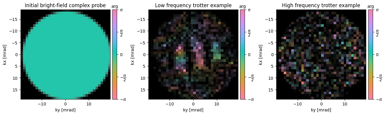
First, notice that our complex overlap trotters look quite different! Notably:
- The phase inside each trotter is not flat, but rather seems to have texture
- The triple-overlap region is no-longer cancelled out
ssb = ssb.reconstruct(
).visualize(
)

reconstructed_object_aberrated = ssb.object.copy()
100%|██████████| 1024/1024 [00:01<00:00, 1136.31it/s]
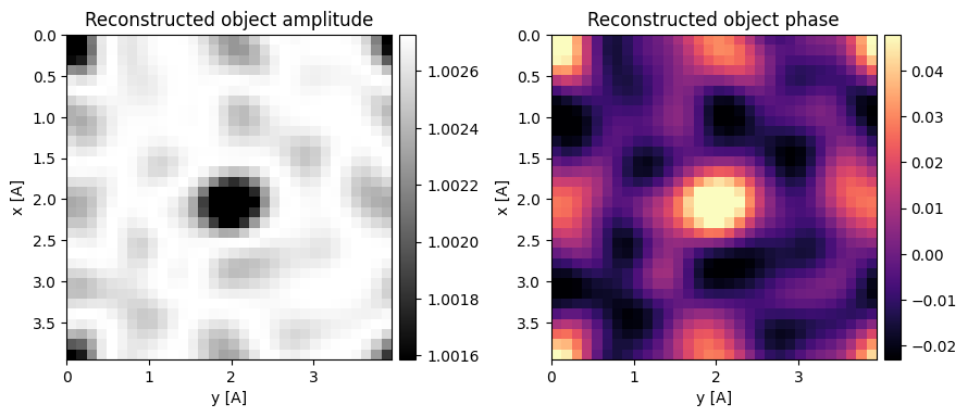
As we expected, the reconstructed object has all-sorts of artifacts.
Optional: Try and correct the aberrations manually!
If you’re feeling brave (and have ipywidgets installed), try correcting the aberrations manually!
# import ipywidgets
# from IPython.display import display
# def widget_wrapper(
# defocus,
# stig,
# stig_angle,
# coma,
# coma_angle,
# trefoil,
# trefoil_angle
# ):
# ssb._verbose = False
# ssb.reconstruct(
# polar_parameters={'C10':-defocus,'C12':stig,'phi12':np.deg2rad(stig_angle),'C21':coma,'phi21':np.deg2rad(coma_angle),'C23':trefoil,'phi23':np.deg2rad(trefoil_angle)},
# progress_bar=False,
# num_jobs=1,
# ).visualize(
# )
# ssb._verbose = True
# style = {'description_width': 'initial'}
# layout = ipywidgets.Layout(width="400px",height="30px")
# kwargs = {'style':style,'layout':layout,'continuous_update':False}
# defocus_slider = ipywidgets.FloatSlider(value = 0,min = -100,max = 100, description = "defocus [Å]",**kwargs)
# stig_slider = ipywidgets.FloatSlider(value = 0,min = 0,max = 100, description = "stig [Å]",**kwargs)
# stig_angle_slider = ipywidgets.FloatSlider(value = 0,min = 0,max = 90, description = "stig angle [°]",**kwargs)
# coma_slider = ipywidgets.FloatSlider(value = 0,min = 0,max = 10000, description = "coma [Å]",**kwargs)
# coma_angle_slider = ipywidgets.FloatSlider(value = 0,min = 0,max = 180, description = "coma angle [°]",**kwargs)
# trefoil_slider = ipywidgets.FloatSlider(value = 0,min = 0,max = 10000, description = "trefoil [Å]",**kwargs)
# trefoil_angle_slider = ipywidgets.FloatSlider(value = 0,min = 0,max = 60, description = "trefoil angle [°]",**kwargs)
# def set_solution(*args):
# defocus_slider.value, stig_slider.value, coma_slider.value, trefoil_slider.value,trefoil_angle_slider.value = (100,0,0,10000,27.5)
# solutions_button = ipywidgets.Button(description='reveal solution!',**kwargs)
# solutions_button.on_click(set_solution)
# output = ipywidgets.interactive_output(
# widget_wrapper,
# {
# 'defocus':defocus_slider,
# 'stig':stig_slider,
# 'stig_angle':stig_angle_slider,
# 'coma':coma_slider,
# 'coma_angle':coma_angle_slider,
# 'trefoil':trefoil_slider,
# 'trefoil_angle':trefoil_angle_slider,
# }
# )
# display(
# ipywidgets.VBox(
# [
# ipywidgets.HBox([defocus_slider,solutions_button]),
# ipywidgets.HBox([stig_slider,stig_angle_slider]),
# ipywidgets.HBox([coma_slider,coma_angle_slider]),
# ipywidgets.HBox([trefoil_slider,trefoil_angle_slider]),
# output
# ]
# )
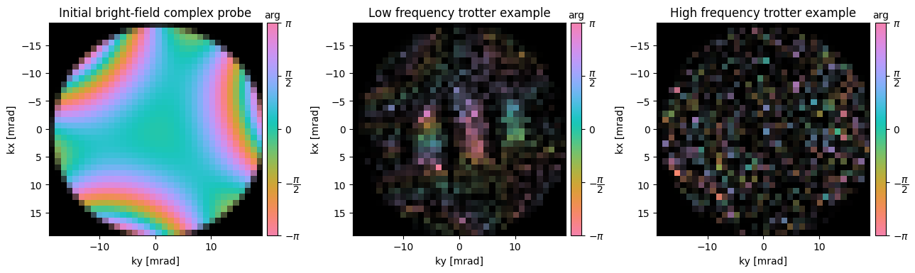
# )Known aberrations reconstructions
Note that similar to how we deconvolved the geometric effects of the probe in the first tutorial, if we know our probe aberrations we can also account for them:
ssb_known = py4DSTEM.process.phase.SSB(
    energy=energy,
    datacube=dataset,
    semiangle_cutoff=semiangle_cutoff,
    C10=-100,C23=10000,phi23=np.deg2rad(27.5),
    verbose=True,
).preprocess(
    plot_center_of_mass=False,
    plot_rotation=False,
    force_com_rotation=-15,
    vectorized_com_calculation=False,
)
Calculating center of mass: 100%|██████████| 1024/1024 [00:00<00:00, 15993.47probe position/s]
Best fit rotation forced to -15 degrees.
Normalizing amplitudes: 100%|██████████| 1024/1024 [00:02<00:00, 464.32probe position/s]
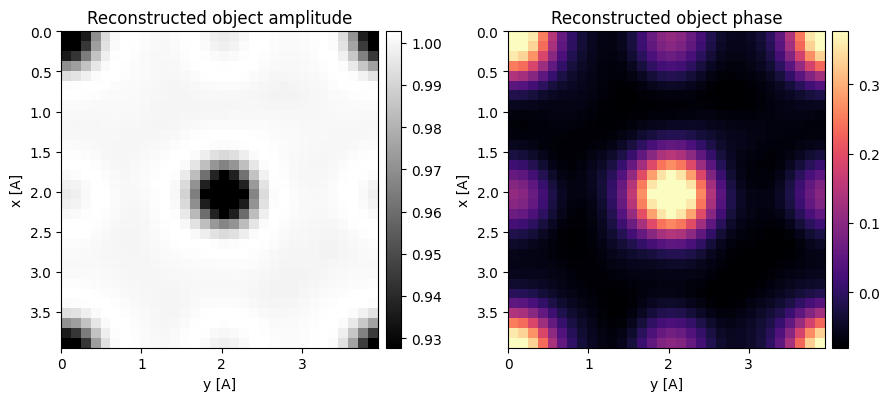
ssb_known = ssb_known.reconstruct(
).visualize(
)

reconstructed_object_known = ssb_known.object.copy()
100%|██████████| 1024/1024 [00:01<00:00, 1000.33it/s]
Estimating aberrations
Our task therefore reduces to estimating the probe aberrations from the dataset directly. Once we know them, we can proceed as usual!
In the parallax_02.ipynb tutorial, we demonstrate one way of doing so using the apparent shifts in virtual bright-field images.
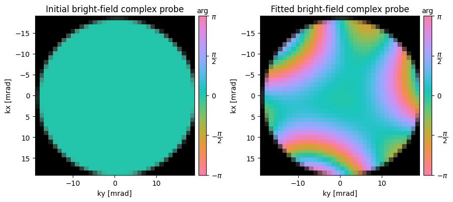
Here, we demonstrate another way by fitting the texture in the complex probe overlaps directly, following 10.1038/ncomms12532.
In particular, we’ll select the 12 trotters with the highest intensity, and fit a basis function of specified order:
ssb = ssb.aberration_fit(
    num_trotters=18,
    max_radial_order=3,
    method='global',
)
Fitted aberration coefficients
--------------------------------------------------
aberration radial angular angle magnitude
name order order [deg] [Ang]
---------- ------- ------- ----- ---------
C1 2 0 --- -102
stig 2 2 -82.9 12
coma 3 1 119.3 5560
trefoil 3 3 25.9 11603
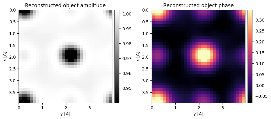
ssb = ssb.reconstruct(
    # polar_parameters=ssb._fitted_polar_parameters, # this is implied when aberration_fit() has ran
).visualize(
)

reconstructed_object_fitted = ssb.object.copy()
100%|██████████| 1024/1024 [00:00<00:00, 1278.31it/s]
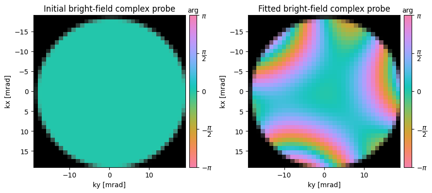
Recursive fitting
The fitting procedure above performed quite well! For noisier datasets, it is often useful to fit the aberration coefficients recursively, i.e.:
- Iteration 1: defocus, stig
- Iteration 2: defocus, stig, coma, trefoil
- Iteration 3: defocus, stig, coma, trefoil, spherical, stig2, quadrafoil,
- Iteration 4: ...
ssb = ssb.aberration_fit(
    num_trotters=12,
    max_radial_order=3,
    method='recursive',
)
Fitted aberration coefficients
--------------------------------------------------
aberration radial angular angle magnitude
name order order [deg] [Ang]
---------- ------- ------- ----- ---------
C1 2 0 --- -113
stig 2 2 -73.3 8
coma 3 1 121.1 5412
trefoil 3 3 25.5 12132
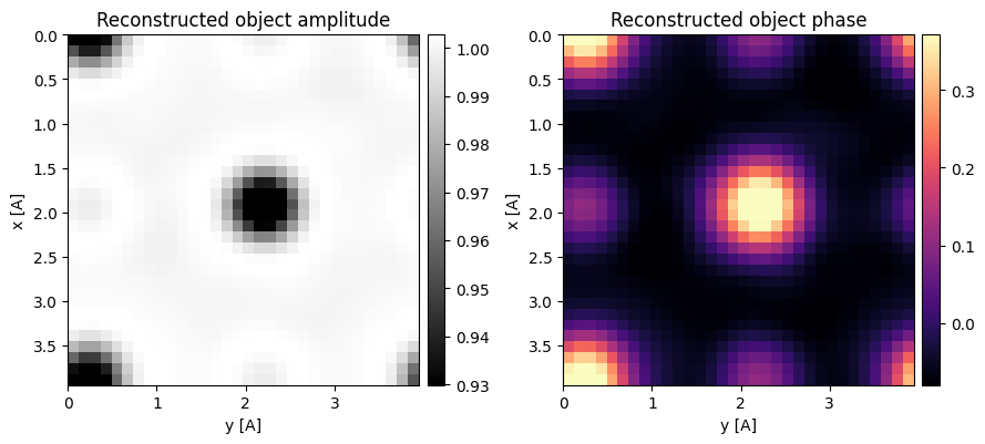
ssb = ssb.reconstruct(
).visualize(
)

reconstructed_object_fitted_recursive = ssb.object.copy()
100%|██████████| 1024/1024 [00:00<00:00, 1201.73it/s]
fig, axs = plt.subplots(1,4,figsize=(16,4))

for ax, arr, title in zip(
    axs,
    (reconstructed_object_aberrated,reconstructed_object_known,reconstructed_object_fitted,reconstructed_object_fitted_recursive),
    ('aberrated reconstruction','known aberrations reconstruction','global fitted aberrations reconstruction','recursive fitted aberrations reconstruction')
):
    py4DSTEM.show(
        np.tile(np.angle(arr),(2,2)),
        figax=(fig,ax),
        cmap='turbo',
        ticks=False,
        title=title,
    )

fig.tight_layout()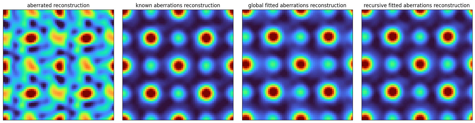
Acknowledgments
This tutorial was created by the py4DSTEM phase_contrast team:

