Armed with our numerical scattering potentials (the “object”) and our incident electron wavefunction (the “probe”), we are now ready to simulate our STEM measurements.

In this section we will introduce the most popular way of simulating electron scattering experiments, the multislice method, introduced by Cowley & Moodie (1957). In Bloch Wave Algorithm, we introduce an alternative approach better suited for periodic calculations of small unit-cells.

Scaled Schrödinger equation¶

Our starting point is the time-independent Schrödinger equation introduced in Scattering Potentials:

where recall $V(\bm{r})$ is the crystal potential and $E$ is the energy of the electron wavefunction $\psi(\bm{r})$.

In the quantum-mechanical wave picture above, we define the De Broglie wavelength (Matter wave) of relativistic free electrons as

where $h$ is the Planck constant, $c$ is the Speed of light, $e$ is the Elementary charge of electrons, and $U_0$ is the accelerating voltage of our microscope’s electron gun.

Source:Multislice Algorithm

energies = np.linspace(20e3,300e3,128)
wavelengths = abtem.core.units.energy2wavelength(energies)

with plt.ioff():
    fig,ax = plt.subplots(figsize=(6,4))
ax.plot(energies/1e3,wavelengths*1e3,color='red')
ax.set(
    xlabel=r"accelerating voltage, $U_0$ [kV]",
    ylabel=r"relativistic electron wavelength, $\lambda$ [pm]"
)
fig.tight_layout()
fig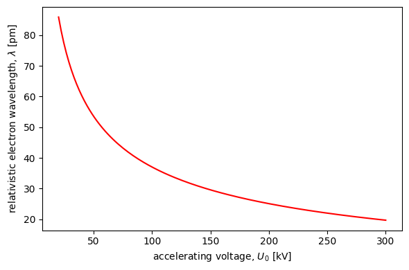

This allows us to define the electron-potential interaction parameter:

and express (3.2) as:

where we have introduced the in-plane electron wavevector, $k_0 = 1/ \lambda(U_0)$. Note this has an implicit dependence on the accelerating voltage, which we omit for notational convenience.

Multislice assumptions¶

To proceed, the multislice method makes two assumptions:

• The $\partial^2 / \partial z^2$ term in the Laplacian can be neglected, since the wavefunction variation along the beam direction (z-axis) is much lower than the in-plane variation
• The in-plane wavevector $k_0$ is much larger than the in-plane variations of the wavefunction, i.e. $k_0 \gg \left| \nabla^2_{x,y}\right|$

Using these assumptions (5.3) can be simplified further to highlight the separation in timescales between the axial and in-plane components Kirkland, 2020:

Equation (5.4) outlines the numerical scheme we will use to solve it. Namely, for a wavefunction $\psi_n$ at a specific depth inside the sample, $z_n$, we can evaluate the operators on the right-hand side over a distance $\Delta z$ to calculate a new wavefunction $\psi_n^{\prime}(\bm{r})$ at position $z_n + \Delta z$.

For small $\Delta z$, the solution to (5.4) is given by Kirkland, 2020:

where

is one slice of the numerical-grid representation of our scattering potential we described in Scattering Potentials.

Split-step Solution¶

Unfortunately, the two operators in (5.5) don’t commute with one another, so a closed-form solution is out of reach. Instead, the multislice method solves (5.5) numerically, by alternating between solving each of the two operators independently.

Transmission Operator¶

Assuming an infinitesimally thin potential slice, we can drop the $\nabla^2_{x,y}$ term in (5.5) to obtain the solution Kirkland, 2020:

where we have defined the transmission operator, $t_n(\bm{r})$. Intuitively, this can be understood as the electron wavefunction acquiring a positive phase-shift proportional to the scattering potential in a particular slice.

Propagation Operator¶

In the next half-step, we need to propagate the electron wavefunction from one slice to the next using (5.5). Setting the space between the slices empty, $V(\bm{r})=0$, and Taylor expanding, we obtain:

Equation (5.8) simplifies further when expressed in Fourier space, $\Psi_{n+1}(\bm{k}) = \mathcal{F}_{\bm{r}\rightarrow \bm{k}} \left[ \psi_{n+1}(\bm{r}) \right]$:

where we have defined the Fresnel propagator, $\mathcal{P}_{\Delta z}(\bm{k})$.

Iterative Fourier Implementation¶

The two propagators can be combined efficiently using the convolution property of the Fourier transform to obtain:

where we have defined the multislice operator, $\mathcal{M}_n$. Equation (5.10) can be applied iteratively until all the potential slices have been traversed, to return the exit wavefunction $\psi_N(\bm{r})$:

Figure 5.1 illustrates the above equations interactively, illustrating the effect of each operator separately. Click somewhere on the potential to position the incoming electron wavefunction, and use the buttons to transmit/propagate the wavefunction through the potential.

Source:Multislice Algorithm

VBox(children=(HBox(children=(Button(button_style='warning', description='transmit', style=ButtonStyle()), But…