Atomic Models
As we saw in STEM Measurements, the first step in simulating STEM measurements is to specify the electrostatic scattering potential of the sample. In the simplest case we will consider in Scattering Potentials, namely the independent atom model (IAM), this is fully specified by the coordinates and chemical symbols of the atoms in the sample.
We will use the Atomic Simulation Environment (ASE) package to manipulate and visualize atomic models of the samples we will simulate.
Periodic unit-cells
The main object of interest in ase is the Atoms class, which defines a collection of atoms.
At a minimum, this can be constructed by passing:
- an array of
Natomic positions in cartesian coordinates with shape(N,3) - a list of
Natomic numbers (or equivalently atomic symbols) - a specification for the periodic unit-cell the atomic coordinates reside in
- e.g. a 6-element list describing the cell lengths and angles
E.g. to create a model for the N2 molecule, we could use
N2_molecule = ase.Atoms(
    positions=np.array([[0.0, 0.0, 0.0], [1.0, 0.0, 0.0]]),
    symbols=["N", "N"],  # "N2" also works
    cell=[6.0, 6.0, 6.0, 90, 90, 90],  # [6.0,6.0,6.0] also works
)
Or the more complicated case of the Si3N4 crystal structure:
Si3N4_crystal = ase.Atoms(
    "Si6N8",
    scaled_positions=[
        (0.82495, 0.59387, 0.75),
        (0.23108, 0.82495, 0.25),
        (0.59387, 0.76892, 0.25),
        (0.40614, 0.23108, 0.75),
        (0.76892, 0.17505, 0.75),
        (0.17505, 0.40613, 0.25),

        (0.66667, 0.33334, 0.75),
        (0.33334, 0.66667, 0.25),
        (0.66986, 0.70066, 0.75),
        (0.96920, 0.66986, 0.25),
        (0.70066, 0.03081, 0.25),
        (0.29934, 0.96919, 0.75),
        (0.33015, 0.29934, 0.25),
        (0.03081, 0.33014, 0.75),
    ],
    cell=[7.6045, 7.6045, 2.9052, 90, 90, 120],
    pbc=True
)
We can visualize Atoms objects along various 2D planes using the abTEM.show_atoms() function.
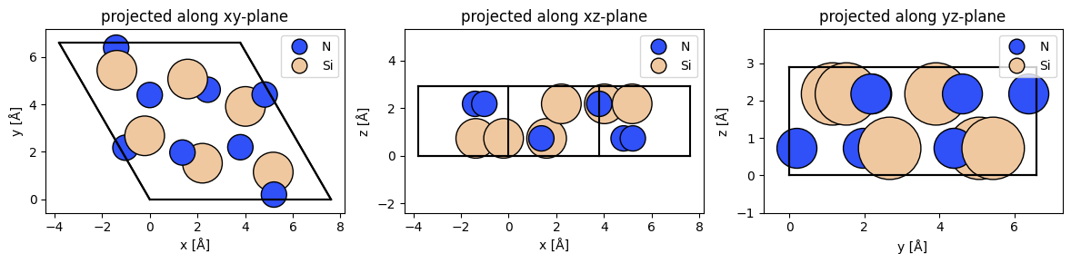
Figure 2.1:Si3N4 unit-cell projected along the three cartesian directions.
Orthorhombic super-cells
We can now use our periodic unit-cell to construct larger “super-cell” structures by tiling along the unit-cell directions.
In ase this is simply achieved by multiplication of the Atoms object.
E.g. Si3N4_crystal * (2,3,1) would return a new Atoms object by tiling the unit-cell twice along the first cell vector, and thrice along the second cell vector.
The multi-slice algorithm we’ll use to simulate STEM measurements requires structures with orthorhombic cells, and thus before we tile our hexagonal unit-cell we need to transform it to an orthorhombic one.
abTEM.orthogonalize_cell is a very convenient function for doing just that.
Si3N4_orthorhombic = abtem.orthogonalize_cell(Si3N4_crystal)
Si3N4_orthorhombic *= (3,2,17)
Here, we are using a (3,2,17) tiling of our orthorhombic unit-cell. This ensures the in-plane cell size is larger than 20 Å x 20 Å, which is usually a safe size to prevent wraparound errors due to periodicity. We choose the tiling along the beam direction to be 17 unit-cells, giving a total thickness of 2.9 Å * 17 = 49.4 Å, i.e. about 5 nm.
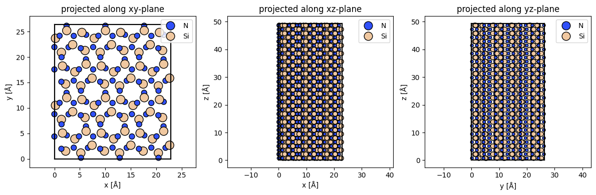
Figure 2.2:Orthorhombic Si3N4 super-cell tiled and projected along the three cartesian directions.
Interactive super-cell widget
Finally, Figure 2.3 illustrates the interactive construction of a SrTiO3 slab with various in-plane dimensions along different zone-axes.

VBox(children=(Canvas(footer_visible=False, header_visible=False, layout=Layout(height='315px', width='675px')…Figure 2.3:Interactive super-cell construction for a Strontium Titanate slab along different zone-axes directions.

